What Function Would You Use to Calculate the Total Number of Periods in a Loan or Investment?
Learning Outcomes
- Utilize financial functions and formulas
Excel provides specific formulas and functions to assist with financial calculations. Nosotros will encompass the top five most oft used financial functions. The post-obit scenario will inform the next example of financial functions.
A person secured a loan from a banking concern to purchase an apartment at an almanac interest charge per unit of six%, over 20 years, with monthly payments. The loan has a present value (PV) of $100,000 (amount of new loan) and a future value (Fv) of 0 (because the goal of the loan is to take it completely paid off at the end of the fourth dimension period). For the monthly payments employ 6%/12 = 0.5% for Rate, and 20*12 = 240 for Nper (total number of payment periods). If only annual payments were made, then it we would use 6% for the Charge per unit and 20 for Nper.
Payment (PMT)
Payment terms for a loan or investment. The Excel formula for it is =PMT(rate,nper,pv,[fv],[blazon]). This assumes that payments are fabricated on a consistent basis.
Follow these steps to find the monthly payment amount for this loan:
- Enter all the information into a table.
- Using the Formulas tab, Financial button, scroll until you find PMT in the drib-downwards menu.
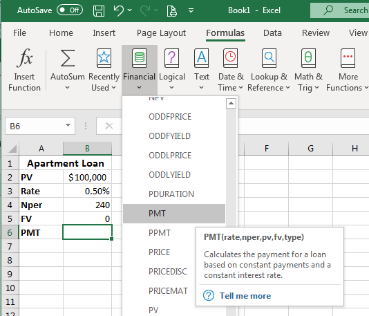
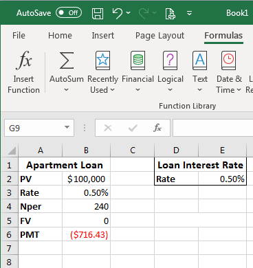
- A dialog window asking for the inputs opens. Click on the cells matching the correct data for that field and the data will be entered into the formula automatically. Using the cell location instead of typing in the direct information, means the formula volition automatically update if new data is entered into those cells. For the last two areas (Fv,Type) for loans, Fv can exist omitted (or enter 0) and Type can also be left empty. Type left empty assumes that payments come up due at the end of the period.
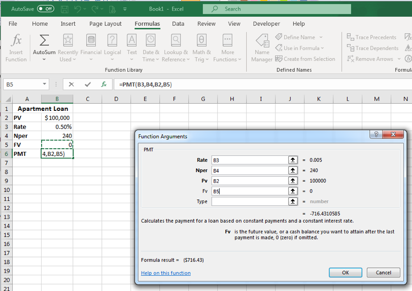
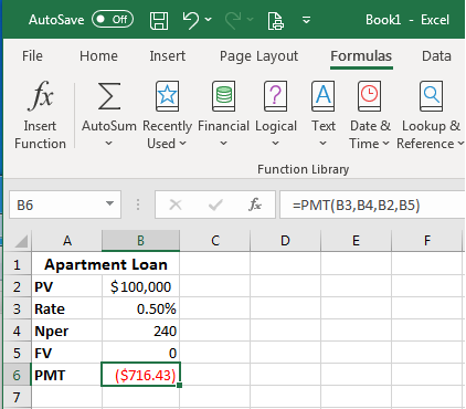
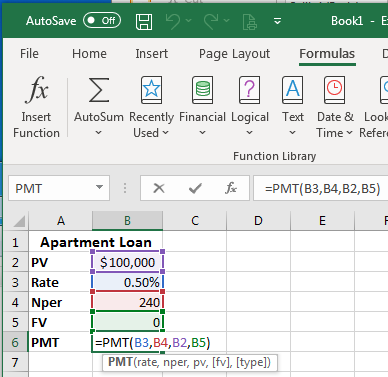
- After the calculation, the monthly loan payment is $716.43. The effigy is crimson because information technology is a debt paid against the total loan. (If you wish to have it not show equally a red/negative number, type in a minus sign before the B2 Rate (-B2) and the PMT will show equally a black, positive number.) The second screenshot shows the PMT formula and the corresponding cells associated with the formula. To see the formula correspondence, double clicking on the jail cell. This correspondence association works with whatever formulas used.
- With the formula established, when y'all modify the rate, present value or nper, yous tin can run across the change in monthly payment information technology will take to pay off the loan.
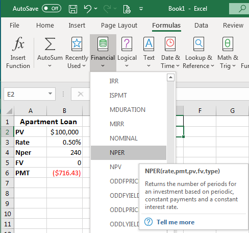
Number of Periods (NPER)
Number of periods per loan or investment. The Excel formula for this is =NPER(rate,pmt,pv,[fv],[type]).
Follow these steps to discover the number of periods for this loan:
- Enter all the information into a tabular array.
- Using the Formulas tab, Financial button, scroll until you lot find NPER in the driblet-down carte.
- A dialog window asking for the inputs opens. Enter the corresponding cell locations.
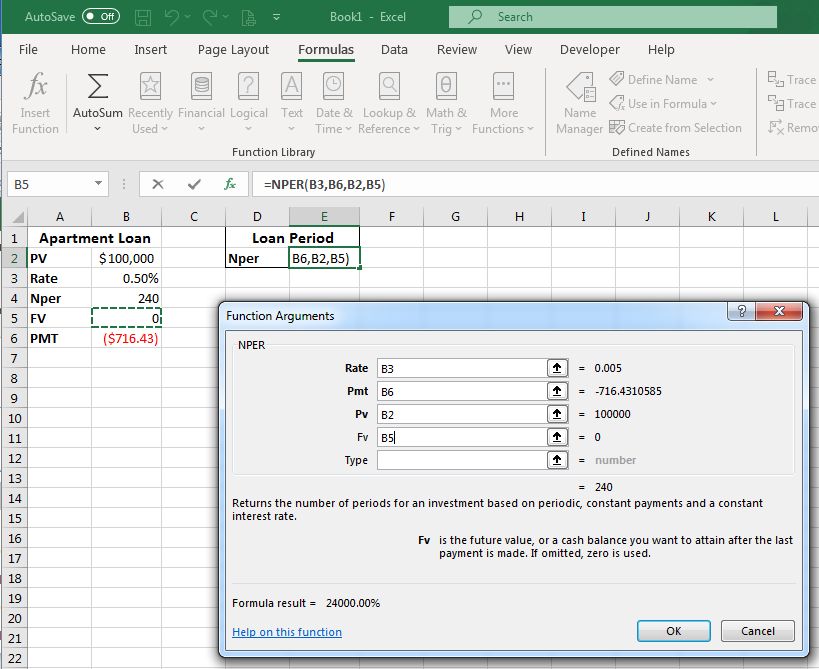
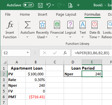
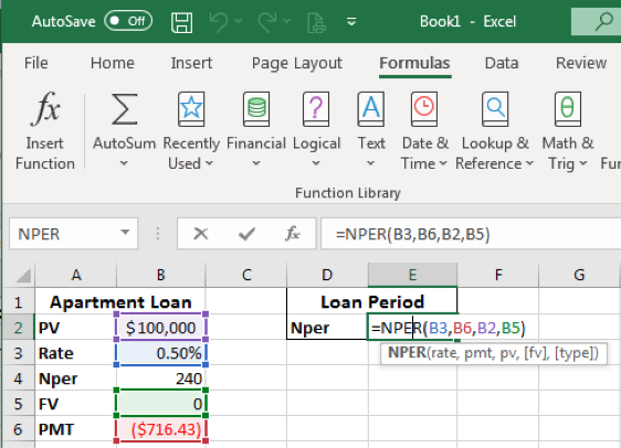
- The Nper is 240 months (20 years of monthly payments). The second screenshot shows the NPER formula and the corresponding cells associated with the formula. Double click on the cell to see its corresponding cells.
- With the formula established, changing the monthly payment corporeality shows the change in the number of periods needed to pay off the loan.
Rate (Charge per unit)
The involvement rate for a loan or a rate of return required to attain a specific amount on an investment over a catamenia of time. The Excel formula for this is =Charge per unit(nper,pmt,pv,[fv],[type],[approximate]). The "guess" for our purposes can be left out for this scenario.
Follow these steps to find the interest rate for this loan:
- Enter all the information into a table.
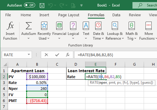
- Using the Formulas tab > Fiscal button > Scroll until you lot observe RATE in the drop-down bill of fare.
- Dialog window opens > Enter the corresponding cell locations.
- The Rate is 0.l%. The second screenshot shows the Rate formula and the corresponding cells associated with the formula. Double click on the prison cell to come across its corresponding cells.
Present Value (PV)
Present value of a loan or investment based on a constant interest charge per unit (like a mortgage or loan). The Excel formula for this is =PV(rate,nper,pmt,[fv],[type]).
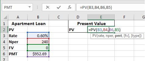
Let's alter the scenario a little to find a PV for a different loan. If yous know that the monthly payments are $952.69, the interest charge per unit is six%, and the life of the loan is 20 years, what is the nowadays value of that loan?
Follow the same steps to insert the formulas like before to find the present value for this loan.
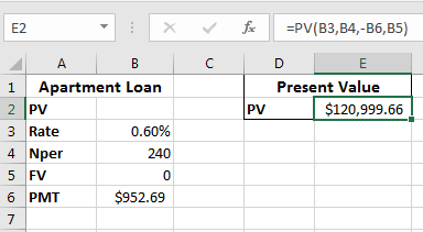
After filling in the values for the in a higher place scenario the PV for this loan is $120,999.66 or if rounded up $121,000.
Future Value (FV)
Future value of an investment assuming constant, periodic payments with a abiding involvement rate. The Excel formula for this is =FV(rate,nper,pmt,[pv],[type]).
Let's alter the scenario once more and discover FV for a dissimilar loan'due south time frame. If you know that the monthly payments are $895.54, the involvement charge per unit is 5%, and the life of the loan is 20 years, is the future value of that loan payed down to 0 in that 20-year time frame?
Follow the same steps to insert the formulas similar before only using the FV part to figure this out.
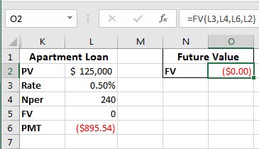
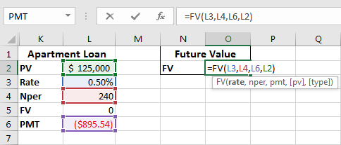
The answer is that, yes, the future value of the loan comes to zero in the timeframe.
Practice Question
Now you lot know how to apply these five financial functions and formulas in Excel.
Contribute!
Did you have an idea for improving this content? We'd honey your input.
Improve this pageLearn More
Source: https://courses.lumenlearning.com/wm-computerapplicationsmgrs-2/chapter/financial-functions-and-formulas/
0 Response to "What Function Would You Use to Calculate the Total Number of Periods in a Loan or Investment?"
Post a Comment